Practical And Business Applications Of Built-In Functions In Ms-Excel 2016 & 2013

One of the attributes of Microsoft Excel that make it unique is its built-in functions that have real life applications both in various fields of study and in business. Some of these built-in functions are: 
• IF functions
• ARITHMETIC functions such as the SUM function, AVERAGE function, etc.
• FORECAST function
• TREND function
• COUNTIF function
• SUMIF function
• CONCATENATE functions

In this chapter, we will explicitly explain these functions with illustrations and real life applications. I will give you some practical exercises to test your knowledge.

This is the first part (Part 1) of this tutorial chapter (Chapter 3). I will illustrate the business applications of various built-in functions in building result system (grade list), payroll systems and how to apply subtotals to these real life systems.

IF FUNCTION ANALYSIS

This is a logical function or conditional statement used to evaluate a given condition. It returns the first variable if the condition is true or met, otherwise it returns the second variable. If the condition is false or not met.

Various application software have IF function as one of their built-in functions with slight difference with this Excel IF function syntax.

The syntax is =IF(condition,[value_if_true],[value_if_false]) Enter

Where;

• Condition is the criteria set for excel to use for the evaluation of the records.
• value_if_true is the variable that will be returned if the condition is met.
• value_if_false is the variable that will be returned if the condition is not met. It is most times ignored.

NESTED IF FUNCTION

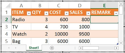
This is a special case of IF function whereby an IF function is enclosed in another IF function. It is used when there are more than one conditions to specify. For example, the worksheet in the figure below contains a table for sales record. In the table, there is a Remark column to contain a remark for each sale. 

If you want Excel to tell you whether you made a profit, loss or you just broke even (I.e. no profit no loss) whenever you enter the item, the quantity sold, the cost price and the selling price, then you will apply a nested IF function in that column.

Place your cursor in cell D2 and type the following nested IF function:

=IF(D2>C2,"profit",IF(D2<C2,"loss",IF(D2=C2,"break even"))) press Enter.

Then use excel fill handle tool to generate a remark for the subsequent cells in the Remark column.

PRACTICAL ILLUSTRATION/BUSINESS APPLICATIONS OF NESTED IF FUNCTION

I will illustrate the various real-life applications of Arithmetic and Nested IF functions of MS-Excel. Please try to practice these examples on your own.

STUDENTS RESULT SYSTEM (GRADE LIST)

QUESTION:

Given that the grade system of Government Secondary School Owerri is as follows:

0 to 39.9 = F

40 to 49.9 = E

50 to 59.9 = D

60 to 69.9 = C

70 to 79.9 = B

80 to 100 = A

Above 100 = Error

If 50 students participated in the examination of the following courses:

Mathematics, English and Biology, using the above grade system, calculate the following for each student:

1. Total score.

2. Average Score.

3. Grades on the respective subjects.

4. Overall grade. 

5. Filter all female students that made an “A” in mathematics.

SOLUTION TO THE GRADE LIST SYSTEM QUESTION

You should first create a table like the one contained in the worksheet in the figure below.

Result System – Table 1

Type in the following formulas in the appropriate cells and use the hand fill tool to generate the results for the subsequent cells in that column:

1. For the TOTAL SCORE column, place your cursor in cell J3 and type the following formula:

=SUM(D3,F3,H3) press Enter.

2. For the AVERAGE SCORE column, place your cursor in cell I3 and type the following formula:

=J3/3 press Enter. Reduce the number of decimals to two.

3. For the ENGLISH GRADE column, place your cursor in cell E3 and type the following formula:

=IF(D3<40,"F",IF(D3<50,"E",IF(D3<60,"D",IF(D3<70,"C",IF(D3<80,"B",IF(D3<=100,"A",IF(D3>100,"ERROR"))))))) press Enter.

4. For the MATHEMATICS GRADE column, place your cursor in cell G3 and type the following formula:

=IF(F3<40,"F",IF(F3<50,"E",IF(F3<60,"D",IF(F3<70,"C",IF(F3<80,"B",IF(F3<=100,"A",IF(F3>100,"ERROR"))))))) press Enter.

5. For the BIOLOGY GRADE column, place your cursor in cell I3 and type the following formula:

=IF(H3<40,"F",IF(H3<50,"E",IF(H3<60,"D",IF(H3<70,"C",IF(H3<80,"B",IF(H3<=100,"A",IF(H3>100,"ERROR"))))))) press Enter.

6. For the OVERALL GRADE column, place your cursor in cell G3 and type the following formula:

=IF(F3<40,"F",IF(F3<50,"E",IF(F3<60,"D",IF(F3<70,"C",IF(F3<80,"B",IF(F3<=100,"A",IF(F3>100,"ERROR"))))))) press Enter.

The completed Grade List System is shown below. 

Result System – Table 2

7. Create the three ranges of data. Type “Female” in the Sex column under the criteria range. Type “A” in the Mathematics Grade column under the criteria range.

Use the procedure for performing Advance filter to filter the database based on the specified criteria.

You might need to revisit chapter 2 for the procedure in advance filter.

PAYROLL SYSTEM DESIGN IN EXCEL

This is the compilation or list of workers’ information and their payment details in an organization or company. It is a database containing all workers information and their payment details such as basic salary, allowances, gross pay, and net pay.

DEFINITION OF SOME TERMS USED IN PAYROLL MANAGEMENT

1. PAY SLIP:

This is a detached leaflet or a record from the payroll that contains a worker’s information and payment details.

2. BASIC SALARY:

This is an amount or sum of money a worker is entitled to at the end of the month in a company or organization which is highly influenced by worker’s qualifications and level, and also by the strength of the organization.

3. ALLOWANCE:

This is a fringe benefit that is allocated to every worker in order to encourage workers and enhance their performance in the company or organization.

4. TAX:

This is a compulsory levy that is deducted from a worker’s basic salary at the end of the month in order to generate revenue for the state and federal government.

5. GROSS PAY:

This is the summation of or the total of a worker’s basic salary and all the allowances he is entitled to at the end of every month.

6. NET PAY:

This is Gross pay minus all deductions such as tax and loans. It is the final take-home of a worker at the end of the month.

PRACTICAL ILLUSTRATION OF A PAYROLL SYSTEM

QUESTION: 

The manager of JOE-LINKS SERVICES wants to computerize the payroll system of the company. As a spreadsheet expert, design a payroll system to his recommendation and approval to pay his workers on monthly basis such that basic salary is influenced by qualification as follows:

WASSCE = $20,000

OND = $25,000

NCE = $28,000

HND = $32,000

BSc = $40,000

MSc = $50,000

PhD = $80,000 respectively.

Marital allowance would be 8% and 10% for single and married workers respectively. Transport, Feeding, Dressing and Housing allowances would be 6%, 4%, 5%, and 8% of their basic salaries respectively.

Compute a tax deduction such that: 

WASSCE = 5%, OND = 6%, NCE = 8%, HND = 10%, BSc = 12%, MSc = 15% and PhD = 20% of their basic salaries respectively.

Calculate the Gross pay and Net pay for each worker.

Setup an advanced query or filter to filter all the married workers with qualification of BSc.

SOLUTION TO THE PAYROLL SYSTEM

You should first create a table like the one contained in the spreadsheet in the figure below:

Payroll System – Table 1

Type in the following formulas in the appropriate cells and use the hand fill tool to generate the results for the subsequent cells in that column:

1. For the BASIC SALARY column, place your cursor in cell D3 and type the following formula:

=IF(C4="WASSCE",20000,IF(C4="OND",25000,IF(C4="NCE",28000,IF(C4="HND",32000,IF(C4="BSc",40000,IF(C4="MSc",50000,IF(C4="PhD",80000,0))))))) press Enter.

2. For the MARITAL ALLOWANCE column, place your cursor in cell E3 and type the following formula:

=IF(B3="Single",D3*8%,IF(B3="Married",D3*10%,0)) press Enter.

3. For the TRANSPORT ALLOWANCE column, place your cursor in cell F3 and type the following formula:

=D3*6% press Enter.

4. For the FEEDING ALLOWANCE column, place your cursor in cell G3 and type the following formula:

=D3*4% press Enter.

5. For the DRESSING ALLOWANCE column, place your cursor in cell H3 and type the following formula:

=D3*5% press Enter.

6. For the HOUSING ALLOWANCE column, place your cursor in cell E3 and type the following formula:

=D3*8% press Enter.

7. For the TAX column, place your cursor in cell J3 and type the following formula:

=IF(C3="WASSCE",D3*5%,IF(C3="OND",D3*6%,IF(C3="NCE",D3*8%,IF(C3="HND",D3*10%,IF(C3="BSc",D3*12%,IF(C3="MSc",D3*15%,IF(C3="PhD",D3*20%,0))))))) press Enter.

8. For the GROSS PAY column, place your cursor in cell K3 and type the following formula:

=SUM(D3:I3) press Enter.

9. For the NET PAY column, place your cursor in cell L3 and type the following formula:

=K3-J3 press Enter.

The completed Payroll System is shown below. 

Payroll System – Table 2

10. Create the three ranges of data. Type “Married” in the M Status column under the criteria range. Type “BSc” in the Qual column under the criteria range.

Use the procedure for performing Advance filter to filter the database based on the specified criteria.

You might need to revisit chapter 2 - part 1  for the procedure in advance filter.

SUBTOTAL AND HOW TO APPLY IT IN AN EXCEL WORKSHEET

Subtotal is an Excel tool used to calculate the total value or amount spent in a particular group of records in a database. It is mainly used in Payroll and Budget Control Systems to calculate the total amount spent in each department of a company.

To Apply Subtotal to a Database in an Excel Worksheet:

1. Prepare and activate the worksheet containing the database you wish to use, for example, a payroll database.

2. Sort the records using the Department column as your sorting field by clicking Sort located in the Sort & Filter group in the Data tab. Select the sort column from the Sort By drop down menu and click OK as shown below.

Subtotal sort

3. Click on Subtotal located in the Outline group of Data tab. The subtotal dialogue box appears.

4. Specify the changing field from the AT EACH CHANGE IN drop down menu which in this case should be the Department column.

5. Specify the ADD SUBTOTAL TO field. In the case of a payroll system, specify either the Gross Pay or the Net Pay column depending on your intention.

6. Put a check the Replace current subtotals and Page break between groups boxes and click OK as shown below. 

Subtotal dialogue

Excel does the calculation for you and returns the values in a row below the last record in each group as shown below.

SOME SAMPLE QUESTIONS UNDER GRADE LIST SYSTEM AND PAYROLL SYSTEM

Please attempt these sample questions:

1. Government Secondary School Owerri wants to computerize her students result in the following subjects:

English, Mathematics, Chemistry, Physics, Biology, Economics, Literature and Government.

a.) As a Spreadsheet Manager, design a result System to compute the Total Score and Average Score.

b.) Using IF function, generate the grade letters for each subject and the overall grade using the following grade Scheme:

0 – 39.9 = Fail

40 – 49.9 = Pass

50 – 59.9 = Credit

60 – 69.9 = Upper Credit

70 – 100 = Distinction

c.) Generate 30 records and Set up an advance filter to filter Science Students from Imo State.

2. a.) Zenith Bank PLC wants to computerize her worker’s payroll system to compute the Basic Salary based on the following qualifications:

SSCE = $1200

NCE = $1300

HND = $1500

BSc = $1800

MSc = $2200

PhD = $2800

b.) Compute 8%, 12%, 7.5%, 6% and 5% of the Basic Salary as Housing, Transport, Medical, Feeding and Dressing allowances.

c.) Tax deduction should be calculated as follows:

SSCE = 1.5%

NCE = 2%

HND = 2.5%

BSc = 3%

MSc = 3.5%

PhD = 4%

d.) Calculate the Gross and Net Pay.

e.) Set up a subtotal to calculate the total amount spent in each department.

This is the end of this part.

Now go over to the next part of this tutorial chapter:

REGRESSION ANALYSIS USING THE FORECAST AND TREND FUNCTIONS

If this tutorial post helped you, then it will also help your friends. Kindly click the one of the share buttons to share this post with your friends.

Don’t forget to subscribe to get our latest tutorial  post delivered to your email.