How To Create A Drop-Down Menu List For A Worksheet Column In Ms Excel – Easy Guide

Creating a drop down list for a worksheet column is very useful especially if you have to type the same data or range of values into different cells of a worksheet over and over again. It makes you type less. When you set up a dropdown menu or list for your columns, MS Excel inserts a dropdown arrow beside each cell in that column. All you have to do is to click the dropdown arrow and select one of the options in the menu. In this tutorial, I will show you a simplified easy guide on how to create or remove a drop down list for a worksheet column.

For example, if in a sales record worksheet, the cells in the PRODUCT NAME column must contain one of the following items: keyboard, scanner, joystick, CPU and mouse, in order to save yourself from the stress retyping these items over again, you prepare a dropdown menu list for that column and then select any of the items from the menu using Excel data validation tool which allows you set some rules to limit the type of data that would be entered in a particular column or call.

This is part 3 of chapter 7 of the Free Online Excel Tutorial Series at Microsoft Tutorial website. In the previous part (part 2), I explicitly explained how to insert data into a worksheet using the data entry form in MS Excel. Also see the full tutorial course content of this Microsoft Excel Tutorial Series.

To Create a Drop Down Menu for a Column in MS Excel:

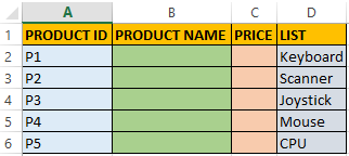
1. Prepare your worksheet like the one shown below.

2. Highlight the entire column B by placing your cursor on the “B” label and clicking when you see the down pointing arrow.

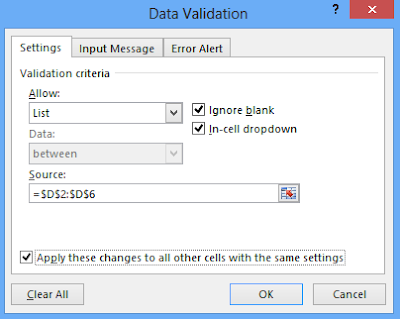
3. Click the Data Validation drop down arrow located in the Data tools group under the Data tab. Then click Data Validation from the resulting dropdown menu option. This prompts the Data Validation dialogue box.

4. Click the Allow: drop down arrow and select List from the resulting options. This activates the Source text box. Type the cell reference of the cells containing the list items. In the above illustration, the list items are contained in column D (cell D2 to cell D6). So type D2:D6 or click the quick selection bolt located at the extreme end of the textbox. Clicking this bolt takes you back to your worksheet. 

Then highlight cells D2 to D6 and then click the minimized quick selection bolt again to return to dialogue box again. You will notice that Excel has automatically generated the absolute cell references (i.e. $D$2:$D$6) of the highlighted cells as shown below.

NOTE:

In a case where there is no column that contains the menu list item, you will type them directly under the Source text box separating each item with a comma and a space. 

5. Check the check box which says: Apply these changes to all other cells with the same settings

6. Click OK to exit the Data Validation dialogue box.

Excel add a drop down arrow beside each cell in column B as shown below. 

You will notice that each cell in column B, including cell B1 has a drop down arrow when activated. But you don’t want a drop down list for cell B1 because it contains the column title.

To Remove the Drop Down Arrow from the Cell Containing the Column Title:

1. Highlight the cell containing the column title and call up the Data Validation dialogue box using the above listed procedure.

2. Select Any Value from the Allow: drop down menu but don’t check any checkbox. Then click OK.

MS Excel removes the dropdown arrow with its menu from cell B1.

To make your workbook more dynamic, you may wish to hide the column which contains the list item (that is column D).

To Hide the Column:

1. First, highlight the entire column.

2. Click the Home tab and then click Format drop down arrow located in the Cells group. Click Hide & Unhide, a sub-option under the Visibility option as shown below.

3. Click Hide Columns and click OK.

NOTE:

The shortcut for hiding columns in MS Excel is Ctrl + 0. To un-hide a column, press Ctrl + Shift + ).

The shortcut for hiding rows in MS Excel is Ctrl + 9. To un-hide a row, press Ctrl + Shift + (.

This is the end of part 3 of chapter 7 of this online tutorial series.

In the next part (part 4), I will explain how to create a drop down menu list for a column in MS Excel.

Was this tutorial helpful to you?

Inform your friends about this post by clicking the share button below. Comment below if you are hooked up along the installation process.

Also click Here to subscribe for free so that you will get our latest game updates in your email.