User Interface And Worksheet Operations In Microsoft Excel (Chapter 1 – Part 2)

Getting used to the various excel worksheet operations will help you work faster and professionally design powerful spreadsheet applications in any available version of Microsoft Excel. In this part I will explicitly explain the hidden excel interface and features and worksheet operations.

This is the second part of this chapter. It is recommended that you first read part one before reading this part. If you have not read part read part one, click to read Part 1: Introduction to MS-Excel.

Click to read - Part 3: Business Applications of Functions in Microsoft Excel.

  CONTENTS

• THE MS-EXCEL USER INTERFACE
• APPLICATION AREAS OF MS-EXCEL
• BASIC TOOL OF MS-EXCEL
• THE DIFFERENCE BETWEEN A SPREADSHEET WORKBOOK AND A WORKSHEET
• WORKSHEET TERMINOLOGIES
• TYPES OF CELL RANGE
• WORKSHEET OPERATIONS
• SAVING YOUR WORKBOOK FOR THE FIRST TIME (SAVE AS)
• RETRIVING A FILE
• CHOOSING OR CHANGING A DATA FORMAT FOR YOUR COLUMNS
• DATA ENTRY

You can download the pdf e-book file of this chapter for free and study at your convenient time. The e-book contains both parts of this chapter properly written. Click to download the e-book: Fundamentals of MS-Excel Using MS-Excel – 2016, 2013,2010 and 2007.

THE MS-EXCEL USER INTERFACE

The MS-Excel user interface is made up of many components as shown below. Study the diagram and its labels.

MS-Excel User Interface

APPLICATION AREAS OF MS-EXCEL

MS-Excel has numerous application areas, but there are three basic application areas of MS-Excel. They include:

• Calculations
• Graphics Management
• Database Management

BASIC TOOL OF MS-EXCEL

The basic tool of MS-Excel is the WORKSHEET. This is because all the MS-Excel works and processes involve a worksheet.

THE DIFFERENCE BETWEEN A SPREADSHEET WORKBOOK AND A WORKSHEET

Most Spreadsheet Mangers and users find it very difficult to differentiate between a workbook and a worksheet. As a result, they use it interchangeably.

SPREADSHEET WORKSHEET

This is where you type, calculate and store data in MS-Excel. It comprises of gridlines of columns and rows. A worksheet contains 256 columns, labeled from A – Z, AA – ZZ, BA – BZ, etc. and 65536 rows labeled from 1 – 65536.

SPREADSHEET WORKBOOK

This is an MS-Excel file where you work and store your data. Each workbook can contain many worksheets. It can have different types of worksheet i.e. can have a sales data worksheet and also have a chart workbook. 

NOTES
By default, a workbook in MS-Excel version 2010 and below has three worksheets. These sheets are named sheet 1, sheet 2 and sheet 3 by default. Each of these sheets has a tab located at the bottom left of the workbook window. You can add another sheet by clicking on the new sheet tab next to the last sheet. You can also delete and insert a worksheet in between existing worksheets. To achieve any of them, right-click on the worksheet left to where you wish to insert the new sheet and click insert > worksheet or delete as the case may be.

Excel 2010 worksheets

In MS-Excel 2013 and 2016, a workbook has only one worksheet named sheet one by default. This sheet has a tab located at the bottom left of the workbook window. To add a new worksheet, click one new sheet as shown below. You can also insert in between worksheets following the procedure listed in the last paragraph.

Excel 2013 and 2016 worksheets

WORKSHEET TERMINOLOGIES

1. CELL: This is an intersection of rows and columns where data is stored.
2.  CELL ADDRESS: This is a descriptive name given to a cell for reference purpose. For example, the first cell in a workbook (i.e. the intersection of column 1 and row 1) is given a cell address of A1.
3. CELL ENTRIES: These are data in form of values and labels stored within a cell.
4. CURRENT OR ACTIVE CELL: This is the particular cell you are working on, which is always highlighted by a cell pointer.
5. CELL POINTER: This is a rectangular bar that always highlights or selects the active cell.
6. CELL RANGE: This refers to two or more selected cells which can be formatted, edited, printed or deleted.

TYPES OF CELL RANGE

There are three types of cell range. They include:

• Vertical or columnar cell range: This refers to selection within a column.  For example, to highlight cells A1 to A10, type =A1:A10 in the formula bar or simply click on the first cell and drag all over to the last cell as shown below.

Vertical cell range

• Horizontal or row cell range: This refers to selection within a row. For example, to highlight cells A1 to E5, , type =A1:E1 in the formula bar or simply click on the first cell and drag all over to the last cell as shown below.

Horizontal cell range

• Rectangular cell range: This refers to selection between rows and columns. For example, to highlight all the cells between cells A1 to E5, type =A1:E5 in the formula bar or simply click on the first cell and drag all over to the last cell as shown below.

Rectangular cell range

DEPENDENT CELL

This is the cell that contains the formula that refers to other cells. For example, if B2 contains the formula =D5,, cell B2 is a dependent cell of cell D5.

PRECEDENT CELL

This is a cell that is being referred to by a formula in another cell. For example, if cell B2 contains the formula =D5, cell D5 is a precedent cell of cell B2.

EXCEL WORKSHEET OPERATIONS

These are the touches or manipulations made on a worksheet in order to make it attractive, presentable, unique and dynamic.

INSERTING A CELL

There may be need to add a new cell between two existing cells in a worksheet. 

To achieve that:

1. Position the cursor on the cell whose immediate left side you desire to add the new column.
2. Click the home tab.
3. Click the drop down arrow under the insert menu in the cells group
4. .Click insert cells and select shift cells right.
5. Click OK.

INSERTING A COLUMN

There may be need to add a new column between two existing columns in a worksheet. 

To Insert a Column:

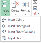
1.    Position the cursor on the column whose immediate left side you desire to add the new column.
2.    Click the home tab.
3.    Click the drop down arrow under the insert command in the cells group.
4.    Click insert sheet columns. Excel inserts the column.
5.    Click OK.

INSERTING A ROW

To insert a row between to existing rows in a worksheet:

1.    Position the cursor on the column whose immediate top you desire to add the new row.
2.    Click the home tab.
3.    Click the drop down arrow under the insert menu in the cells group.
4.    Click insert sheet rows. Excel inserts the row.

DELETING A ROW OR A COLUMN

To delete a row or a column from a worksheet:

1.    Position the cursor on the row or column you wish to delete.
2.    Click the home tab.
3.    Click the drop down arrow under the delete menu in the cells group.
4.    Click delete sheet rows or delete sheet columns as the case may be. Excel deletes the row or column.

INSERTING A WORKSHEET

To insert a worksheet in between existing worksheets:

1.    Activate the worksheet whose immediate left you wish to insert the new worksheet.
2.    Click the home tab.
3.    Click the drop down arrow under the insert menu in the cells group.
4.    Click insert sheet.

DELETING A WORKSHEET

To delete a worksheet:

1.    Activate the worksheet you wish to delete.
2.    Click the home tab.
3.    Click the drop down arrow under the delete menu in the cells group.
4.    Click delete sheet.

RENAMING A WORKSHEET

To rename a worksheet:

1.    Activate the worksheet you wish to rename.
2.    Click the home tab.
3.    Click the drop down arrow under the format menu in the cells group.
4.    Click rename sheet, a sub-option under the Organize Sheet option. The default sheet name located at the bottom left is highlighted.
5.    Type in a new name for the sheet and press enter key to commit it.

HIDING A WORKSHEET

For some reasons you may not want a particular worksheet in your workbook to be visible to everybody who opens that workbook. In such situations, you hide that worksheet. 

To hide a worksheet:

1.    Activate the worksheet you wish to hide.
2.    Click the home tab.
3.    Click the drop down arrow under the format menu in the cells group.
4.    Hover your mouse pointer on Hide & Unhide, a sub-option under the Visibility option. Then click on Hide Sheet. Excel hides the worksheet so that it is no more visible.
5.    Type in a new name for the sheet and press enter key to commit it.

NOTE: 

You can also hide a cell, column, rows or selected rows and columns using the same procedure.

UNHIDING A WORKSHEET

To unhide a worksheet you hid previously:

1.    Click the home tab.
2.    Click the drop down arrow under the format menu in the cells group.
3.    Hover your mouse pointer on Hide & Unhide, a sub-option under the Visibility option. Then click Unhide Sheet. Excel displays a list of hidden worksheets.
4.    Select the worksheet you wish to unhide and click OK.

Unhide dialogue box

NOTE: 

You can also unhide a cell, column, rows or selected rows and columns using the same procedure.

FREEZING A ROW OR COLUMN

If a certain row or column is an object of identification for the rows of your table, you may wish to make it static on the worksheet screen. When you freeze a row or column, Excel moves the column to the extreme left with a thick line separating it from other rows and columns.

To freeze a row or column:

1.    Activate the worksheet that you wish to hide its row or column.
2.    Click the view tab.
3.    Click the drop down arrow under the Freeze Panes menu in the window group.

Freeze pane menu

4.    Click Freeze top row or Freeze first column depending on your aim. Excel freezes the column or row.

UNFREEZING A ROW OR COLUMN

To unfreeze a row or column:

1.    Activate the worksheet that you wish to hide its row or column.
2.    Click the view tab.
3.    Click the drop down arrow under the Freeze Panes menu in the window group.
4.    Click Unfreeze panes depending on your aim. Excel unfreezes all previously frozen column or row.

CHANGING YOUR WORKSHEET BACKGROUND

To change your worksheet background:

1.    Activate the worksheet you wish to change its background.
2.    Click the Page Layout tab.
3.    Click Background menu in the Page Setup group. Excel prompts the Browse sheet background dialogue box. Select a background picture from your PC and click Insert.

NOTE: In Excel 2013 and 2016, an alert pops up if your PC is offline notifying you that you need an internet connection to us online background picture.

Background picture alert

Just click Work offline to select background picture from your PC.

 USING THE AUTO FILL (FILL HANDLE)

The auto fill is one of the features of Excel used to fill the subsequent cells in a column with respect to the data you entered in the first cell or row. For example, if you wish to fill a particular column with the months of the year or you are performing calculation in a column, all you need to do is type the first month (i.e. January) or type the formula in the first cell depending on your choice, auto fill will fill up the rest of the cells with the correct data. 

To use auto fill:

1.    Type the first or the formula as the case may be on the first cell and press the enter key.
2.    Position the cell pointer on that first cell to make it active.
3.    Move the mouse pointer to the lower right corner of the cell pointer (it resembles a square dot). This spot is called a fill handle. Once the mouse pointer reaches this spot, it changes to a small addition sign (+).
4.    Click and drag to highlight all the subsequent cells you wish to auto fill the value, then release the mouse button. Excel fills these cells with the correct data with respect to the data or formula in the first cell as shown below.

Auto fill

CREATING A BORDER OR GRIDLINE

MS-Excel does not create an automatic border around your worksheet. Borders are very necessary especially if you intend to print your work. 

To create a border round your work:

1.    Highlight the entire cells to contain the border
2.    Click the home tab.
3.    Click the drop down arrow below Format as table menu in the styles group.
4.    Select any table design of your choice.

Border Designs

USING THE CONDITIONAL FORMATTING

Excel now has a feature that helps you to automatically format cells, rows, columns or group of rows and columns that match a criterion (e.g. cell ranges a particular data type, etc.). The conditional formatting menu is located in the styles group under the home tab. You can choose from the pre-defined rules or create your own rule.

The conditional formatting menu

PAGE LAYOUT OPERATION

This operation is very necessary especially for works you intend to print. It configures your wok to fit the printout paper size. You can choose the print themes or templates, margins, orientation size area, etc. 

To layout your page:

1.    Activate the worksheet you wish to print.
2.    Click the Page Layout tab.
3.    Make some necessary adjustments to your work for a neat printout.

Page Layout

MERGING AND CENTERING YOUR HEADINGS

The merge and center command is used to centralize your titles or headings over cells. It also converts several cells into a single cell and centralized any data in the merged cells. Also note that you should only merge and center empty cells. 

To merge and centralize a group of cells:

1.    Highlight the cells you wish to merge.
2.    Click the home tab.
3.    Click the merge and center icon in the alignment group. Excel merges those cells to a single cell.
4.    Now type in your title in the merged cell. Excel also centralizes your title. In the cell.

Merge and Center

TRANSPOSING YOUR DATA OR INFORMATION

Transposing of data means converting data from column wise to row wise. For example, if you have a data in a particular row which you also need in a particular column, you don’t need to retype it. Excel can help you do that easily. 

To transpose data:

1.    Highlight the data you wish to transpose
2.    Click the home tab.
3.    Click the copy command icon in the clipboard group.
4.    Position your cell pointer on the first cell of the column or row you want the data to be.
5.    Click the drop down arrow under the paste command menu icon.
6.    Click Paste Special.

Data transpose

7.    From the resulting options check the Transpose sub-option under Operation option and click OK. Excel transposes the data for you.

SAVING YOUR WORKBOOK FOR THE FIRST TIME (SAVE AS)

To save your workbook:

1.    Click the file tab.
2.    Click Save As.  This prompts the save as dialogue box.
3.    Specify any save location or destination of your choice (e.g. document, desktop).
4.    Type the file name you wish to give your workbook and click the save button.

RETRIEVING A FILE

To retrieve a file you have previously created in Excel:

1.    Click the file tab.
2.    Click Open. This prompts the Open dialogue box.
3.    Locate your save location or destination (e.g. document, desktop).
4.    Select the file you wish to open by selecting the file name and click the open button.

NOTES: In Excel 2013 and 2016, you can check some recent files or click Computer icon, then click browse for file icon to locate your save location.

Retrieving files

HOW TO PASTE SPECIAL IN EXCEL

The paste special command in excel helps you to copy a cell or cells data together with the source formatting and formulas and also updates the cell references in the formulas with reference to the new location.

When you just copy and paste a cell’s data to a new location, Excel returns the #REF error message because you copied a formula with invalid cell references.

To Copy and Paste special in Excel: 

1. Activate the cell containing the data you want to copy.

2. Right click and click Copy.

3. Activate the new cell location (Where you want to paste the copied data).

4. Right click and click Paste Special from the resulting menu.               

Then the Paste Special dialogue box appears.

5. Under Paste Options at the top, select Values option. 

6. Click Ok. You should now see the value in the new cell location.

The Paste Special command saves you a lot of time especially when you have a lot of calculated values to paste.

CHOOSING OR CHANGING A DATA FORMAT FOR YOUR COLUMNS

In MS-Excel, you can choose different data format for different columns depending on the type of data to be stored in them. For example you can set date format for a column that stores date data and currency format for a column that stores currency. Other formats include: General, Number, Accounting, Percentage, Scientific, Text, etc. The General format is the default format i.e. when none is specified. 

To choose or change data format for a column:

1.    Activate or highlight the column you wish to choose or change its data format by clicking on the column label e.g. column A, column B, etc.
2.    Click the drop down arrow in the Number group located in the Home tab pane and select any format of your choice. You can also select different currency types by clicking the drop down arrow near the dollar sign ($) located under the first drop down arrow in the Number  group as shown below.

Changing or choosing a data format

DATA ENTRY
The worksheet accepts two major kinds of data. They include: values and labels.

Labels are titles in form of alphabets in a cell. They are always left justified while values are numbers ranging from 0 to 9. They are always right justified. See the illustration below.

Data entry

This is the end of part two of this chapter.

Click to read - Part 3: Business Applications of Functions in Microsoft Excel.

Feel free to share this tutorial with your friends. See you in the next part of this chapter.